
2D GUI Tutorial
The 2D GUI fits and simulates Bayesian causal inference models in experiments
where each stimulus has two dimensions. A common example is an audiovisual
numerosity task in which each trial contains both numerosity information
(Flash and Beep) and temporal information (SOA).
Launch the 2D GUI
import bcitoolbox as btb
btb.gui2d()
Equivalent aliases are also available:
btb.gui_2d()
btb.twoD()
getattr(btb, "2D")()
Home Screen
The 2D GUI opens with three modules:
- Model Fitting
Fit one or more CSV datasets, compare decision strategies, visualize behavioral and model-predicted response distributions, and export figures or CSV summaries.
- Simulation
Simulate a single 2D continuous condition and preview the response distribution in real time.
- About
Citation, contact, and model background information.
Data Format
Each row should represent one behavioral trial. The default CSV format is:
Flash |
Beep |
SOA |
R_F |
R_B |
|---|---|---|---|---|
1 |
1 |
0 |
1 |
1 |
1 |
2 |
150 |
1 |
2 |
2 |
1 |
300 |
2 |
1 |
2 |
2 |
500 |
2 |
2 |
0 |
1 |
0 |
1 |
|
1 |
0 |
1 |
0 |
FlashandBeepPrimary-dimension stimuli for modality 1 and modality 2. In the default audiovisual numerosity case, these are visual flashes and auditory beeps.
SOASecondary-dimension disparity. By default, the GUI interprets this as modality 1 minus modality 2.
R_FandR_BParticipant responses for modality 1 and modality 2.
- Missing unimodal values
Use
0for a missing modality stimulus. The GUI automatically treats the unavailable secondary value as missing during model evaluation.
You can create this template directly from the GUI by clicking
Save suggested format. A small example file is also available here:
demo_2d.csv.
Column Mapping
The Data format panel allows the same model to be used across multiple
experimental designs.
- Dimensions
Choose
Numerosity + Time,Spatial + Time, orSpatial + Numerosity. The choice updates parameter labels and recommended default ranges.- Modality 1 and Modality 2
Choose labels such as
VisualandAuditory. These labels appear in plots and exported files.- Secondary input
Choose how the secondary dimension is represented:
Single disparity column: modality 1 minus modality 2Single disparity column: modality 2 minus modality 1Single disparity column: centeredTwo modality-specific columns
- Column selectors
Map each model variable to the corresponding CSV column. After importing a file, the GUI reads the header row and fills the dropdown menus with the detected column names.
Fitting Settings
SimulationsNumber of Monte Carlo samples per condition. Use
1000for a quick check and10000or higher for final analysis.Random seedsNumber of independent seed initializations. More seeds increase robustness and computation time.
Fit typemllcomputes a likelihood-based objective and enables log likelihood, AIC, and BIC output.minusr2andsseprovide descriptive distribution-matching objectives.ToolPowellis the default optimizer.VBMCcan be selected when pyvbmc is available in the active environment.StrategiesSelect one or more of
ave,sel, andmat. If multiple strategies are selected, the GUI fits each strategy and reports the best-fitting one for each dataset.
2D Parameters
Parameter |
Meaning |
Default role |
|---|---|---|
|
Prior probability that the two modalities come from a common cause. |
Free by default |
|
Sensory uncertainty for the primary dimension in modality 1 and 2. |
Free by default |
|
Sensory uncertainty for the secondary dimension in modality 1 and 2. |
Fixed by default |
|
Prior standard deviation and mean for the primary dimension. |
Free by default |
|
Prior standard deviation and mean for the secondary dimension. |
Fixed by default |
|
Additive response bias for modality 1 and 2. |
Fixed by default |
The visible labels change with the selected dimensions and modalities. For
example, sigma_v_number may appear as sigma Visual numerosity.
Run a Batch Fit
Open
Model Fitting.Click
Import CSV filesand select one or more datasets.Confirm the column mapping.
Choose dimensions, modalities, secondary-input mode, fit type, optimizer, and strategies.
Review free parameters and bounds.
Click
Run batch fitting.Watch the output panel for seed-level optimization progress and final parameter estimates.
The GUI stores the best result for each imported dataset in memory until the window is closed or a new batch is run.
Inspect and Export Results
Visualize datasetOpens a figure comparing behavioral response probabilities with model predictions for each condition.
Save all figuresSaves one
*_2d_bci_fit.pngfigure per dataset.Save prediction CSVExports condition-level behavioral and model-predicted response probabilities. This is the best file for custom plotting or reporting model checks.
Save fitting summary CSVExports one row per dataset with error, log likelihood, AIC, BIC, number of free parameters, number of observations, selected strategy, optimizer, seed, dimensions, modalities, and fitted parameter values.
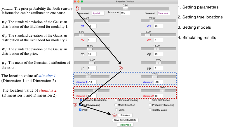
Simulation Tutorial
Open Simulation from the home screen to preview the 2D model without
loading a dataset.
Select the dimension pair and modality labels.
Choose the decision strategy.
Enter the stimulus condition: modality 1 primary, modality 2 primary, modality 1 secondary, and modality 2 secondary.
Edit parameter values.
Click
Run simulationor wait for the live preview to update.Click
Save simulated CSVto export simulated responses.
The simulation figure displays the stimulus locations, modality-specific response clouds, density contours, and peak or mean response estimates. This view is useful for checking whether a fitted parameter set produces plausible 2D behavior before running a large batch analysis.
Best Practices
Verify the CSV mapping after import, especially when column names differ across experiments.
Start with a small number of simulations while checking data formatting.
Use multiple random seeds for final analyses.
Keep parameter bounds scientifically plausible for the unit of measurement.
Report the strategy set, fit objective, number of simulations, number of seeds, free parameters, and exported AIC/BIC values when applicable.
Use
mllwhen likelihood-based information criteria are needed.